Source code for Christmawave

If you follow my podcast, you’ll note I put out a vaporwave-ish Christmas album, Christmawave. It’s a free download on Bandcamp, but I’m asking those who can afford it to donate to the Hackney Winter Night Shelter.

Almost all of the pieces are constructed using variations on one algorithm. I found hoary, old baby boomer Christmas favourites and then took the instrumental sections, which was sometimes just the intro or the outro. All of the songs were in 4/4 and most of the instrumental parts where cut into either in 2 or 4 bar phrases. This means every sample is divisible by many powers of 2 and can be cut in half several times before it loses musical/rhythmic meaning.

I made these cuts, played the section of the sample with some stuttering and then went on to another section of the sample. This method requires some decision making:

1. Which sample am I going to play?
2. How many times am I going to divide it in half?
3. Once it’s chopped into little (or not-so-little) pieces, which one of them am I going to play?
4. What speed am I going to play that bit at?
5. How much should it overlap whatever comes after?
6. How long should I wait before going to the next thing (which might be a repetition of what I just did)?
7. How many times should I repeat this thing?

All of the pieces answered these questions in slightly different ways. (Or very different ways, in the case of question 1!) Some of the structuring of how I thought about these questions and how I solved them have to do with how the Pattern library works in SuperCollider.

What sample am I going to play?

In almost every case, I switched samples based on how much time had passed since the start of the piece. I used Ptpars to start different sections.

How many times am I going to divide it in half?

Another way of asking the question is, ‘what power of 2 am I going to use?’ I did this a few different ways. In most cases, I stuffed this into part of the event I called pow. Here are some ways I figured out what power of 2 to use:


\pow, Prand([0, 0, 0, 0, 0, 1, 1], inf)


Then later, on I could go from that to powers of two:


\div, Pfunc({|evt|
2.pow(evt[\pow])
})


(Usually, I would compute the \div in a larger Pfunc that figures out more things.) The advantages of figuring out the power of 2 instead of just having a Prand full of 1, 2, 4, etc are that this is harder to screw up. I don’t need to worry about a stray 3 sneaking in, and, if a sample is longer, I can add some number to the \pow to make the \div bigger.

Another way I computed the \pow was using a Finite State Machine. This was completely overkill, but I’ll walk you through how it worked.

What I wanted was to have a possibility of a \pow being as small as 0 or as big as 8, but not to jump from one of those numbers to the other. Instead, I wanted a route going through intermediate numbers, in which it could potentially get to an 8 and have a path back to 0. I wanted a way for it to wander from one extreme to the other.

A FSM offers a way to give a path. This is what the code looks like from Funky (The Slow Jam):


\pow, Pfsm([
#[0], //start
2, #[3], //0
Prand([0, 0, 1], 1), #[1, 2], //1
Prand([0, 1, 2]), #[1, 2, 3], //2
Prand([1, 2]), #[3, 4], //3
Prand([0, 1, 2]), #[3, 5], //4
Prand([2, 3]), #[4, 3, 5, 6], //5
Prand([3, 4]), #[4, 3, 5, 7], //6
Prand([3, 4, 5]), #[4, 3, 5, 6] //7
], inf),


Pfsm is the pattern library that does state machines. It takes an array. The first item in the array is an array of what states it can start with. Next comes pairs. Each pair is a state. The first pair is state 0. The second pair is state 1. The third pair is state 2, etc. The first item in a pair is the output. In the example above, the output of state 0 is 2 and the output of state 1 is Prand([0, 0, 1], 1).

The second item in the pair is an array of one or more integers. The numbers in the array are the states you can go to next. So with state 0, the array is ‘#[3]’, so it goes on to state 3. When it gets to state 3, it produces the output, which is Prand([1, 2]) and then looks where it can go next, which is ‘#[3, 4]’. That is, it can go state 3 again, or it can go on to state 4.

I could draw a map of this (which would reveal that there is no path to states 1 and 2 – oops).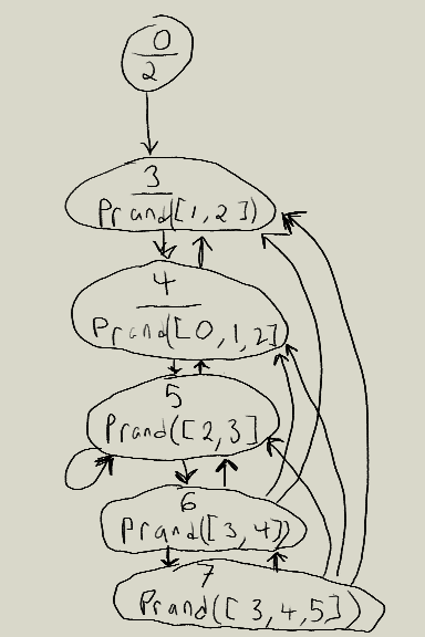

In the graph, you can see a lot of arrows pointing up and few pointing down, only along a path that goes through all the states. Thus, it’s relatively unlikely to reach state 7.

Because Pfsm is just another pattern, I could add 1 or 2 to the output of it in the case of a particularly long sample and it would gracefully handle the maths.

Answers to the other questions will be forthcoming in following posts!