This is the fourth part of a series of posts about how I created my album Christmaswave. Previously, part 1 posted a list of questions and answered the first two of them: ‘What sample am I going to play?’ and ‘How many times am I going to divide it in half?’. Part 2 answered the question, ‘Once it’s chopped into little (or not-so-little) pieces, which one of them am I going to play?’. Part 3 talked endlessly in the meandering way of hangovers about playback rates.
One thing I have not addressed is how I picked which parts of source material to use. Unless the words were compelling in some way, I tended to go for phrases that were instrumental. In some songs, this left me only the intro and the outro. This is why most of the pieces have source material taken from multiple versions of the same song.
How much should an event overlap whatever comes after?
Normally, you would do this by setting the \legato part of the event, which is ‘The ratio of the synth’s duration to the event’s duration.’ I set this to 1.1 in most of the pieces, which helped make up a bit in case the slicing was in slightly the wrong place.
Most I varied:
\legato, Pwhite(0.8, 1.5)
Some depended on the duration of the it of sample I’m playing. This is what I did with Sledge Trudge
\legato, Pfunc({|evt|

	var dur, legato;

	dur = evt[\dur];

	legato = 1;

	(dur < 0.01).if({ legato = 2}, {
		(dur < 0.07). if({ legato = 1.5},
			{legato = 1})
	});
	legato
})
How long should I wait before going to the next thing (which might be a repetition of what I just did)?
This is a question as to what to put for the \dur part of the event, which depends on the number of frames of sample that we're playing, the sample rate of it, and the playback rate.
I pulled a lot of my source material from youtube - by using a browser plugin to download and convert to mp4 and the using audacity to convert to wav files. These files were often 48k, which is the standard for film, but audio is generally at 44.1k, so I did have to take the source file's sample rate into account.
It makes sense to calculate the start frame and duration together. This example is from Out in the Cold:
[\startFrame, \dur], Pfunc({|evt|

	var buf, startFrame, dur, div, start, frames;

	start = evt[\start];

	div = evt[\div];

	buf = evt[\buf];

	frames = buf.numFrames;

	startFrame= frames * (start/div);

	rate =evt[\rate];

	dur = (frames / buf.sampleRate) / rate * div.reciprocal;
[startFrame, dur]
})
How many times should I repeat this thing?
The glitchy repeating of the same event multiple times is a repetition of the entire event, not just some parts of it. I did this with Pclutch, which has a slightly weird syntax.
Pclutch(

	pattern,

	connected

).play
The pattern is just your Pbind or similar, but the connected part is slightly odd. If it's true, the Pbind is evaluated to produce a new value. It's it's false, the previous event is repeated. It's possible to use a pattern to control this.
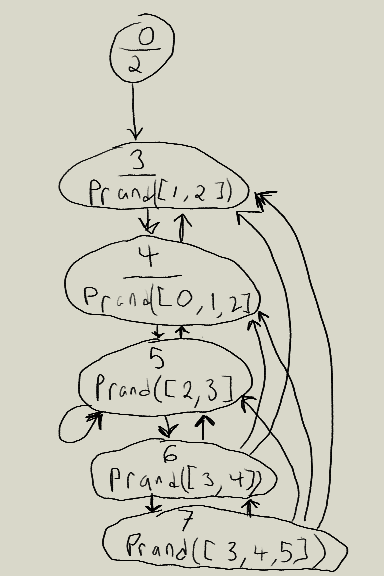
This is the pattern I used for Walking in a Winter No Man's Land. 0 is equivalent to false and 1 is equivalent to true.
Pseq([0, 0, 0, 0, 1,

  Prand([

    Pseq([Pn(0,2), 1],1),

    Pseq([Pn(0, 3),1],1),

    Pseq([Pn(0,4), 1], 1)

  ],100)

])
Starting with the Pseq means that the Pclutch will repeat 4 times, then make a new event. After that, it picks randomly from 3 Pseqs. The first repeats twice, the second 3 times and the third 4 times. It will randomly pick between these repetitions for 100 times and then stop.